Privacy Notice: This website uses analytics and marketing cookies to understand reader behavior and improve content. By continuing to browse or engage with this site, you consent to our use of cookies. See our Privacy Policy for details.
Editor’s Note: With VERDAZO proudly joining Omnira Software in 2022, this blog is being re-published on the Omnira Software website.
The presence of IP30, IP60, IP90 … has increased in recent years. Is this a trend that has evidence to support its growing use? … or is this a trend that should be accompanied with appropriate caution? Let’s find out!
To truly answer this question we need to establish a context for our assessment. This includes:
- Understanding each production measures’ strengths and weaknesses
- Comparing IP values against other production measures
- Use “correlation to EUR” as our “measure of usefulness” (from a reserves perspective)
Another “measure of usefulness” that we can explore in a future blog is the IP correlation to 60 month cumulative production. This is the biggest money making period for horizontal wells and where payout takes place. Some preliminary analysis suggests that the correlations would be dramatically higher than they are to EUR. But let’s get back to today’s focus… we’ll start with the conclusions, then cover the correlation results, followed by the EUR calculation methodology.
Conclusions
When I presented the correlation results to a number of industry professionals, the expectation was that the correlations would be higher. Why weren’t they? Hopefully the following conclusions will help you understand why.
- More data is better: correlations improve as more data is available. This would also improve the reliability of your auto-forecast of EUR.
- Completions matter: the early production of these wells is frac-dominated, transitioning to reservoir dominated flow. The variability in frac designs contributes to lower correlations on large diverse datasets. Including more data improves the correlation.
- Compare apples to apples: the more variability in your dataset (completion design, operator, geology etc.) the lower you can expect your correlation to be. Your correlations will improve with similarity of wells amongst your data set. Poor correlations could be an indicator of the degree of variability in your sample set…. or that there really isn’t a strong correlation. We would expect the correlations shown in this blog to potentially be a “worst case” scenario (i.e. lowest expected correlations due to the broad variability in the dataset))
- Condensing of data helps: when using the Cumulative measures, the exclusion of zero months has only a moderate improvement on the correlations.
- Producing Day (PD Rates) should be used with caution: PD Rates are calculated using producing hours, and as a result introduce another possible source of error. With careful manual culling of PD Rate outliers, the correlation could be improved … but beware of inaccurate reporting of producing hours.
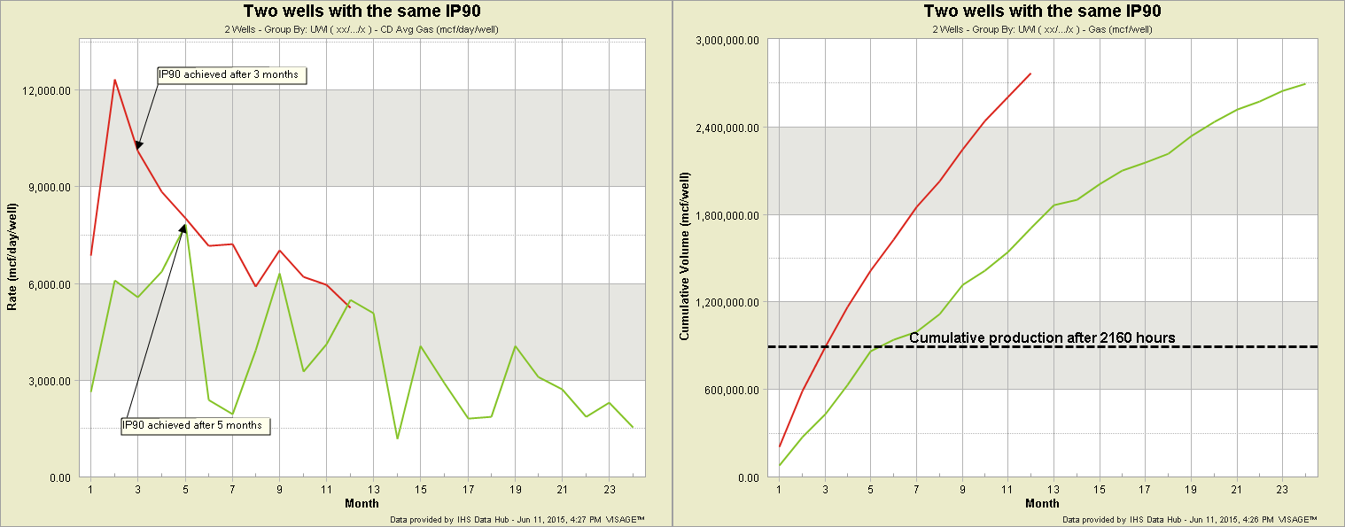
- IP30, IP60, IP90 … should be used with caution: Because IP rates also rely on producing hours, there can be data quality issues that can plague your results. Because IP rates factor out elapsed time, two wells can have the same IP90 with very different production profiles (see charts below). Get to know your data and understand how much downtime your wells have when using IP. Some stats on elapsed time to IP30 are:
- an average of 79 days to get Oil IP30 on a collection of Bakken, Viking and Cardium wells (2578 wells)
- an average of 101 days to get Gas IP30 on a Montney sample set (518 wells)
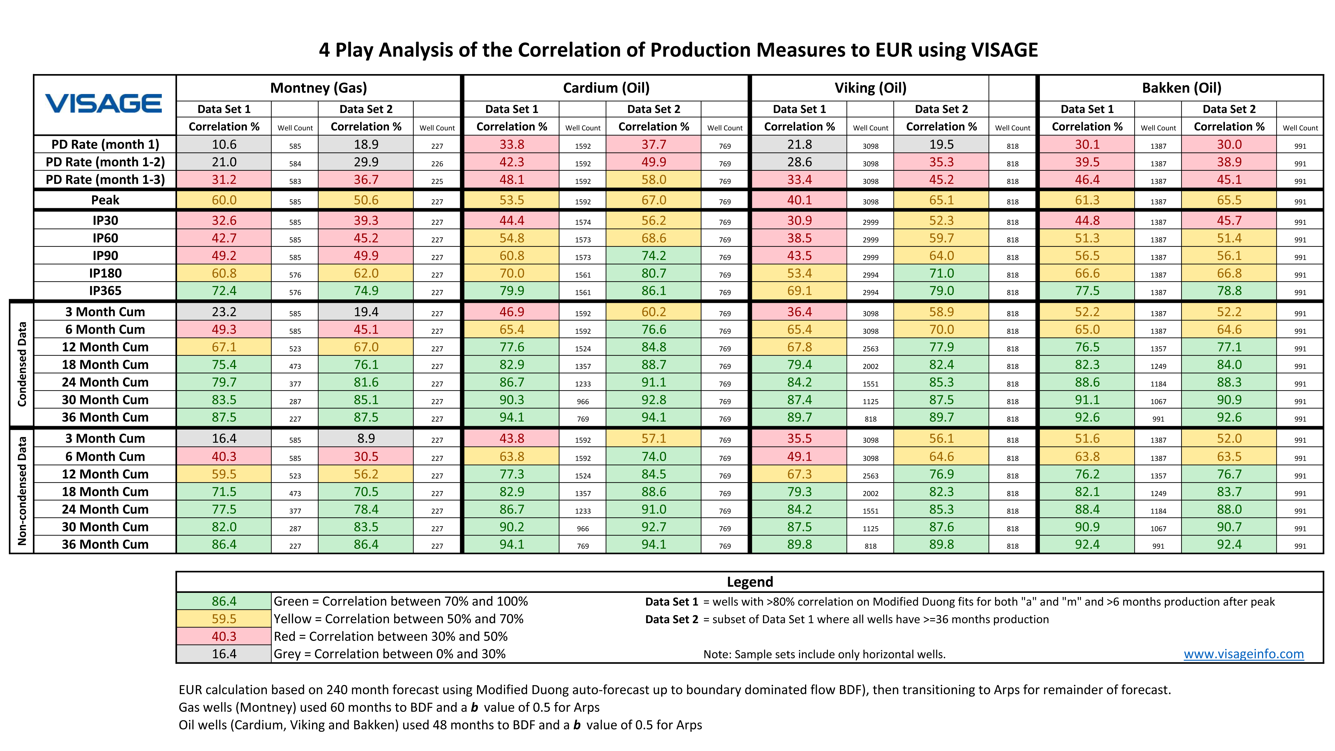
Correlation Analysis Results
EUR Calculations
Datasets
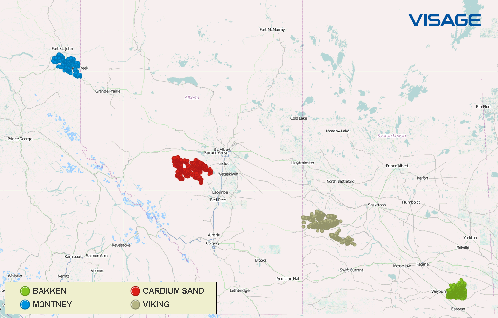
I selected datasets from 4 major plays made up of horizontal wells with more than 6 months of production after peak [Montney (gas), Cardium (oil), Viking (oil), Bakken (oil)]
Forecasting Method
Modified Duong to Arps auto-forecasting was run on all wells using VERDAZO. The resulting dataset was culled to only include wells where both Duong fits for “a” and “m” were greater than 80%. The other parameters used were:
Oil Wells:
- Use Modified Duong up to 48 months (then transition to boundary dominated flow)
- The remaining forecast used Arps with a “b” value of 0.5
- Replaced forecast with actual production values in EUR calculation
- Total EUR forecast was for 240 months
Gas Wells:
- Use Modified Duong up to 60 months (then transition to boundary dominated flow)
- The remaining forecast used Arps with a “b” value of 0.5
- Replaced forecast with actual production values in EUR calculation
- Total EUR forecast was for 240 months
