Editor’s Note: With VERDAZO proudly joining Omnira Software in 2022, this blog is being re-published on the Omnira Software website.

Normalization of data is a means to improve the comparability of wells or groups of wells. Today’s blog will cover three types of normalization:

1) Time Normalization: alignment of time periods (months) relative to a date or event

2) Dimensional Normalization: scaling production values relative to a well design parameter

3) Fractional Normalization: scaling production values relative to the peak rate

Each approach serves a distinct purpose and together they can be used to build an informative narrative.

1) Time Normalization

There are two common dates used to align time, “First Production Date” and “Peak Rate Date”. Each has its own strengths and weaknesses.

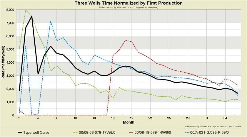
First Production Time Normalization

Strength: on larger well sets, this communicates the average production profile taking into account variability in time to peak. This is suitable for some comparisons (e.g. operator, vintage).

Weakness: the resulting type-well curve may not accurately reflect production decline behavior (as shown in the example below).

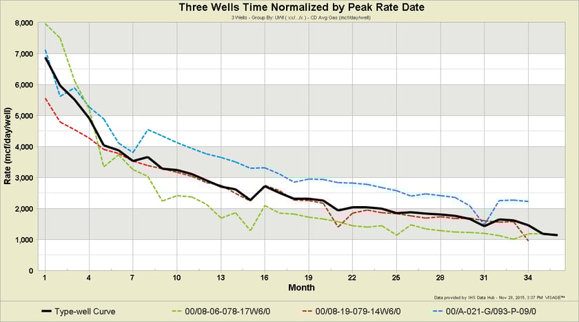
Peak Rate Date Time Normalization

Strength: the type-well curve typically reflects production decline behavior more accurately (as shown in the example below).

Weakness: the type-well curve excludes ramp up time (to peak) which is not important to EUR calculations but is important to first year revenue projections. There are techniques to incorporate ramp up to peak (discussed in the next section of this blog).

Ramp Up to Peak

A statistical approach can be used to derive a type-well curve of the ramp up to peak. It is a two-step process that involves:

i) determining the “typical” time it takes to get to peak

ii) using negative time on the type-well curve to show the ramp up

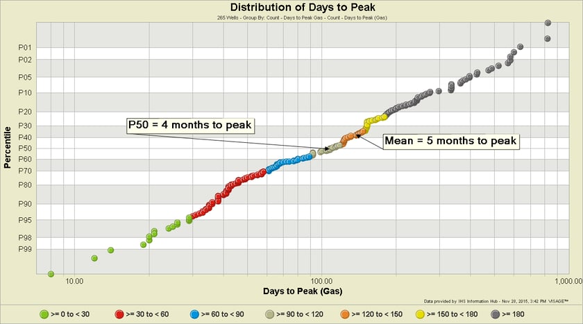
A probit plot of the time to peak (with 30 day bins) is a statistical tool to help you identify a “typical” ramp up time. Time to peak is an approximation due to the nature of monthly data. It is calculated as the end of the month in which peak rate occurred minus the on production date. This example shows that half the wells took less than four months and half took more than four months (i.e. the P50) with a mean of 5 months. Either the P50 or mean value could be used, as long as it is consistent with your operational plans. This chart could also be used to cull your analogue data set… but be cautious not to introduce bias in your analogue well selection. A general rule is “if a well has an outcome that could happen then include that well”.

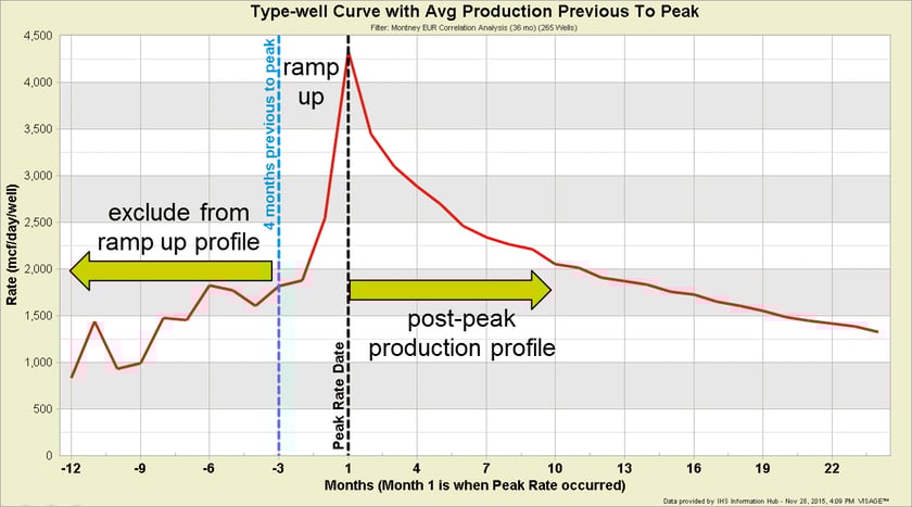
ii) Negative Time Type-well Curve (for ramp up profile)

Having identified a “typical” ramp up time of 4 months (using the P50), I can expose negative time on my Peak-date normalized production profile to reveal a typical ramp up production profile. Any data previous to the 4 month cut-off would be excluded.

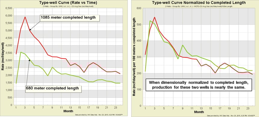
2) Dimensional Normalization

Dimensional normalization typically involves taking a production measure and dividing by a well design parameter. It can be an effective way to rationalize production performance differences between wells. It is also a powerful tool used for completion optimization analysis (an example of this in action can be found in the blog Frac Analysis in VERDAZO: How to Refine Your Insights Using Distributions). The process involves using a dimensionally normalized variable and grouping by other design parameters in an attempt to identify optimal configurations. Common dimensionally normalized variables include:

• Production/Completed Length
• Production/Stage
• Production/Perforation
• Production/Completion Cost
• Production/Tonne of Proppant
• Production/Fluid Pumped (m³)

The following example shows how dimensional normalization can be used to explain the production difference between two wells and illustrates how their production per 100m completed length is nearly the same.

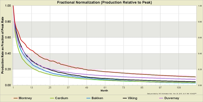
3) Fractional Normalization

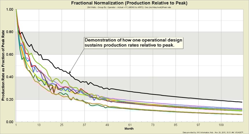
Fractional normalization is a means of expressing production rates relative to peak rate (simply divide any month’s production rate by the peak production rate). Given a peak rate you could apply it to the curve to derive a quick (approximate) production forecast (assuming all peaks deliver the same curve shape). The biggest advantage of this technique is that it allows you to characterize the decline shape and compare plays, companies, technologies, well designs, operational approaches etc. in a common context.

Fractional Normalization Example 1: Comparison of production decline shapes of five different plays

Fractional Normalization Example 2: Comparison of operational designs between several operators

That concludes part 3 of this series. The remaining topics that you can look forward to include:

• Calendar Day vs Producing Day
• Condensing Time
• Operational/Downtime Factors on Idealized Curves
• Survivor Bias
• Truncation Using Sample Size Cut-off
• Forecast the Average vs Average the Forecasts
• Representing Uncertainty
• Auto-forecast Tools

___________________________________________________________

About Bertrand Groulx

Bertrand Groulx is a well-respected oil and gas industry expert with almost 30 years of experience driving innovation and developing advanced solutions. He possesses deep knowledge and understanding of data analytics in the sector, which has allowed him to deliver unparalleled enhancements to Omnira Software's VERDAZO and MOSAIC software products. Bertrand's extensive accomplishments in the public and private sectors and his scientific publications and presentations on machine learning, visual analytics, and completion optimization have made him a thought leader. With a B.S. Honors in Geology and Geology and Geomorphology from the University of British Columbia, Bertrand focuses on enhancing Omnira Software's business intelligence and discovery analytics products in his current role, particularly the VERDAZO platform's growth and development. As a blog author, Bertrand shares his unique expertise and insights, offering valuable knowledge and guidance to industry professionals seeking to stay at the forefront of the constantly evolving oil and gas landscape.

Production data: IHS Information Hub

Completion and Frac Data: Well Completions and Frac Database from Canadian Discovery

Analysis: VERDAZO

Some other blogs you may find of interest:

• Type Curves Part 1: Definitions and Chart Types
• Type Curves Part 2: Analogue Selection
• What production performance measure should I use?
• Frac Analysis in VERDAZO: How to Refine Your Insights Using Distributions

About Bertrand Groulx

Bertrand Groulx is a well-respected oil and gas industry expert with almost 30 years of experience driving innovation and developing advanced solutions. He possesses deep knowledge and understanding of data analytics in the sector, which has allowed him to deliver unparalleled enhancements to Omnira Software's VERDAZO and MOSAIC software products. Bertrand's extensive accomplishments in the public and private sectors and his scientific publications and presentations on machine learning, visual analytics, and completion optimization have made him a thought leader. With a B.S. Honors in Geology and Geology and Geomorphology from the University of British Columbia, Bertrand focuses on enhancing Omnira Software's business intelligence and discovery analytics products in his current role, particularly the VERDAZO platform's growth and development. As a blog author, Bertrand shares his unique expertise and insights, offering valuable knowledge and guidance to industry professionals seeking to stay at the forefront of the constantly evolving oil and gas landscape.